Why Backprop Isn’t Magic: The Challenge of Local Minima

Backpropagation is the cornerstone algorithm powering much of the deep learning revolution. Coupled with gradient descent, it allows us to train incredibly complex neural networks on vast datasets. However, it’s not a silver bullet. One of the fundamental challenges that can prevent backpropagation from finding the best possible solution is the presence of local minima in the optimization landscape.

Backpropagation and Gradient Descent: The Core Idea

At its heart, training a neural network is an optimization problem. We define a loss function, often denoted as $L(\theta)$, which measures how poorly the network performs with its current set of parameters (weights and biases), collectively represented by $\theta$. Our goal is to find the parameter values $\theta^*$ that minimize this loss.

Backpropagation is the algorithm used to efficiently compute the gradient of the loss function with respect to each parameter in the network, $\nabla L(\theta)$. This gradient tells us the direction of steepest ascent in the loss landscape. To minimize the loss, we use an optimization algorithm, typically a variant of gradient descent. The standard update rule for gradient descent is:

Here, $\eta$ is the learning rate, a hyperparameter that controls the size of the step we take in the opposite direction of the gradient. We repeatedly apply this update rule, iteratively adjusting the parameters $\theta$ to descend the loss landscape, hopefully towards a point where the loss is minimal.

Problems During Optimization

Imagine the loss function $L(\theta)$ as a high-dimensional landscape, where the parameters $\theta$ define the coordinates, and the value of the loss function $L$ defines the altitude. Our goal is to find the lowest valley in this entire landscape – the global minimum.

However, the landscapes defined by loss functions for complex models like deep neural networks are rarely simple, smooth bowls (convex). Instead, they are often highly non-convex, featuring numerous hills, valleys, plateaus, and saddle points.

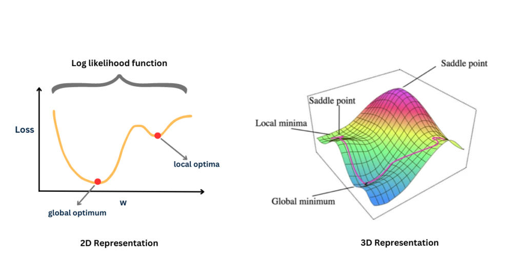[Figure 1] Gradient descent, starting from different points, might end up in different minima. The lowest point is the global minimum, while others are local minima.

The Local Minima Trap

A local minimum is a point $\theta_{local}$ in the parameter space where the loss $L(\theta_{local})$ is lower than at all nearby points, but potentially higher than the loss at the global minimum $\theta_{global}$.

Mathematically, for a point $\theta_{local}$ to be a local minimum, the gradient must be zero: \(\nabla L(\theta_{local}) = 0\) And the Hessian matrix (matrix of second partial derivatives) must be positive semi-definite.

The problem arises because the standard gradient descent algorithm follows the negative gradient downhill. Once it enters the basin of attraction of a local minimum, the gradients will guide it towards the bottom of that specific valley. When it reaches the exact bottom of the local minimum, the gradient becomes zero (or numerically very close to zero). According to the update rule:

The updates stop, and the algorithm converges, getting “stuck” in the local minimum, even if a much deeper valley (the global minimum) exists elsewhere in the landscape.

Example: Consider a simple 1D loss function like $L(x) = x^4 - 5x^2 + 4$. The derivative is $L’(x) = 4x^3 - 10x$. Setting $L’(x) = 0$ gives $2x(2x^2 - 5) = 0$. The critical points are $x=0$, $x=\sqrt{5/2}$, and $x=-\sqrt{5/2}$. Let’s evaluate the loss: $L(0) = 4$ $L(\pm \sqrt{5/2}) = (\sqrt{5/2})^4 - 5(\sqrt{5/2})^2 + 4 = 25/4 - 5(5/2) + 4 = 6.25 - 12.5 + 4 = -2.25$.

Here, $x=0$ is a local maximum (not minimum in this case, but illustrates a point where gradient is zero), and $x=\pm \sqrt{5/2}$ are global minima. A slightly more complex function could easily have multiple points where $L’(x)=0$ corresponding to distinct local minima with different loss values. If gradient descent starts near a suboptimal local minimum, it will likely converge there.

Getting stuck in a local minimum means the trained model is suboptimal – it hasn’t learned the best possible mapping from inputs to outputs according to the chosen loss function and data. Its performance (e.g., accuracy, prediction error) will be worse than a model that managed to find the global minimum or a deeper local minimum.

Can Randomness Help? Randomized Search and SGD

If the landscape is treacherous, how can we improve our chances of finding a good minimum? Introducing randomness is a common strategy.

1. Stochastic Gradient Descent (SGD): Instead of calculating the gradient $\nabla L(\theta)$ using the entire dataset (which is computationally expensive and leads to standard gradient descent), SGD calculates the gradient based on a small, randomly selected subset of the data, called a mini-batch (or even a single data point). \(\theta_{new} = \theta_{old} - \eta \nabla L_{batch}(\theta_{old})\) The gradient computed on a mini-batch, $\nabla L_{batch}(\theta)$, is a noisy estimate of the true gradient $\nabla L(\theta)$. This noise is not necessarily bad! The random fluctuations in the gradient estimate mean that the optimization path is erratic rather than smooth. This inherent noise can help the optimizer “bounce” out of shallow local minima or traverse saddle points more effectively. It doesn’t guarantee finding the global minimum, but it significantly improves the exploration of the loss landscape compared to standard gradient descent.

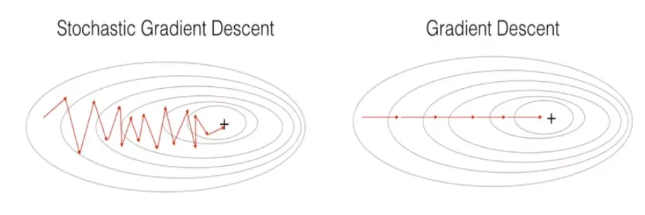[Figure 2] The smooth path of GD potentially likely gets stuck, while the noisy path of SGD might escape a local minimum and find a better solution.

2. Random Restarts: Another approach is to run the entire gradient descent optimization process multiple times, each time starting from a different, randomly initialized set of parameters $\theta$. Since different starting points might lead to different local minima, we can simply pick the model that achieved the lowest loss value across all the runs. This increases the chance of finding a good minimum but comes at the cost of significantly more computation.

3. Advanced Optimizers: Modern optimizers like Adam, RMSprop, and AdaGrad incorporate concepts like momentum and adaptive learning rates. While not purely random search, they often use estimates derived from noisy mini-batch gradients and include mechanisms that help navigate complex landscapes more robustly than vanilla SGD or standard gradient descent, implicitly leveraging the benefits of noisy updates.

Saddle Points vs. Local Minima

Interestingly, recent research suggests that in the extremely high-dimensional spaces typical of deep learning, true local minima might be less of a problem than previously thought. Instead, saddle points – points where the gradient is zero, but which are minima along some dimensions and maxima along others – are potentially more common and problematic. The good news is that the same noisy updates from SGD that help escape local minima are also effective at navigating away from saddle points.

Conclusion

While backpropagation provides the essential gradients, the optimization process itself, usually gradient descent or its variants, faces the challenge of navigating complex, non-convex loss landscapes. Getting trapped in local minima (or stuck near saddle points) can prevent our models from reaching their full potential. Introducing randomness, most notably through the use of Stochastic Gradient Descent (SGD) and randomized search, is crucial in modern deep learning. It helps algorithms explore the parameter space more effectively and increases the likelihood of finding high-performing models, even if it doesn’t always guarantee finding the absolute global minimum.