
Supervised Learning Showdown: kNN, SVM, Neural Networks, and Boosted Trees
Published:
In this post, we dive into the world of supervised learning, comparing the performance of four popular algorithms: k-Nearest Neighbors (kNN), Support Vector Machines (SVM), Neural Networks (NN), and Decision Trees with Boosting (specifically, AdaBoost). We’ll analyze their effectiveness on two distinct datasets, highlighting their strengths and weaknesses.
Datasets
We worked with two datasets in this analysis:
Dataset 1: Fetal Health Classification
This dataset focuses on fetal health monitoring during pregnancy and childbirth. It includes 21 features extracted from Cardiotocography (CTG) exams, such as fetal heart rate and uterine contractions. The goal is to classify fetal health into three classes: Normal, Suspect, and Pathological. This dataset comprises 2,126 instances and features an imbalanced class distribution, with the Normal class having a much larger representation than other classes. This presents challenges for some models.
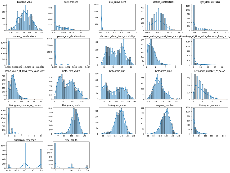
As seen in [Figure 1], several features exhibit skewed distributions and the target variable, fetal_health, has an imbalanced class distribution. Furthermore, the histogram_width feature has very high variance, so it is excluded from the modeling to simplify them.
Dataset 2: Sleep Health and Lifestyle Dataset
The second dataset explores the link between sleep habits and lifestyle factors. It contains data from 400 individuals with 13 features such as sleep duration, physical activity, stress levels, and cardiovascular metrics. This dataset also includes information on sleep disorders, which serves as our target variable. We converted the target variable into a binary classification problem: presence of any sleep disorder (Insomnia or Sleep Apnea) vs. absence of a disorder. This resulted in a more balanced dataset. The original target included 3 categories: none, insomnia, sleep apnea.
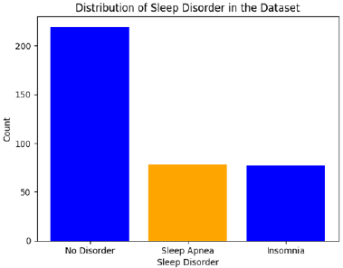
[Figure 2] depicts the distribution of sleep disorders within this dataset. The “No Disorder” category is the largest, with fewer instances of Sleep Apnea and Insomnia.
Several categorical features in this dataset were one-hot encoded to create binary variables in order to work well with the models.
Hypotheses
Before diving into the implementation, we established a few key hypotheses:
- Sample Size Impact: We expected models trained on the larger fetal health dataset (Dataset 1) to exhibit better generalization performance and be less prone to overfitting compared to models trained on the sleep dataset (Dataset 2).
- Minkowski Distance in kNN: We predicted a higher optimal Minkowski distance (p) value for the kNN model on Dataset 2 due to the higher dimensionality resulting from one-hot encoding of the categorical features.
Methodology
Our methodology involved the following steps:
- Data Preprocessing: We performed an 80:20 train-test split on both datasets.
- Model Implementation: We used scikit-learn, PyTorch, and torchvision to implement our models.
- Baseline Model Training: Initially, all models were trained using default parameters.
- Learning Curve Analysis: We analyzed the learning curves to identify issues such as overfitting or underfitting.
- Hyperparameter Tuning: Using a 3-fold cross-validation approach, we optimized the hyperparameters of each model.
- Final Model Evaluation: The best-performing models from the cross-validation process were evaluated on the held-out test set.
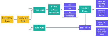
[Figure 3] depicts the experiment process flow, from processed data to the model evaluation.
Model Implementation
k-Nearest Neighbors (kNN)
For kNN, we tuned the number of neighbors (k) using a rule of thumb, then cross-validated against different values. We also experimented with different Minkowski distance metrics using different p values.
Support Vector Machine (SVM)
We explored different kernel functions (linear, polynomial, radial basis function) and regularization parameters during hyperparameter tuning, aiming to balance bias-variance trade-off.
Neural Network (NN)
We started with a basic two-layer NN and then experimented with different architectures (number of layers, neurons, activation functions), as well as dropout and learning rate.
Decision Trees with Boosting (AdaBoost)
We implemented AdaBoost and then optimized hyperparameters like number of estimators, learning rate, and maximum tree depth. We also implemented pre-pruning to improve generalization and reduce overfitting.
Results
| Datasets | Metric | kNN | SVM | NN | Boosted DT |
|---|---|---|---|---|---|
| Dataset 1 | Accuracy | 0.92 | 0.90 | 0.88 | 0.93 |
| Precision Avg | 0.84 | 0.84 | 0.79 | 0.87 | |
| Recall Avg | 0.81 | 0.81 | 0.78 | 0.92 | |
| Dataset 2 | Accuracy | 0.85 | 0.88 | 0.89 | 0.88 |
| Precision Avg | 0.85 | 0.87 | 0.86 | 0.86 | |
| Recall Avg | 0.80 | 0.83 | 0.87 | 0.83 |
[Table 1] summarizes the performance metrics, such as accuracy, precision, and recall for all models with their default settings.
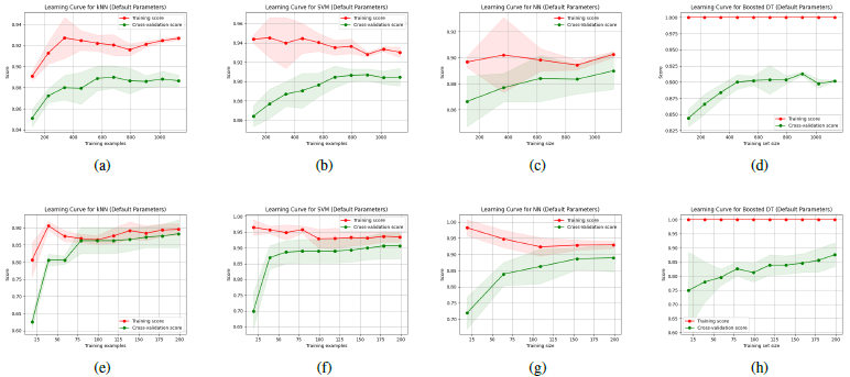
[Figure 4] visualizes the learning curves for the models with default parameters across both datasets. In the plot, red lines indicate the training score, and green lines indicate cross validation score. Shaded areas also represent the variance.
Hyperparameter Tuning and Cross-Validation
| Models | Parameter | Dataset 1 | Dataset 2 |
|---|---|---|---|
| kNN | Number of neighbors | 4 | 4 |
| Minkowski distance metric | 1 | 5 | |
| SVM | C | 10 | 1 |
| Kernel type | rbf | rbf | |
| NN | Hidden layer | (64, 32, 16) | (32) |
| Dropout rate | 0.2 | 0 | |
| Learning rate | 0.1 | 0.01 | |
| Boosted DT | Number of Estimators | 200 | 200 |
| Learning Rate | 0.5 | 0.1 | |
| Max Depth | 2 | 1 | |
| Min Samples Split | 2 | 2 | |
| Min Samples Leaf | 1 | 1 |
[Table 2] reports the tuned hyperparameters of each model.
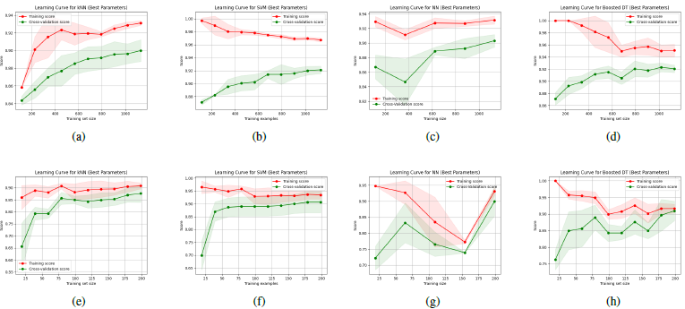
[Figure 5] illustrates the learning curves of the models after hyperparameter tuning.
Key findings from hyperparameter tuning:
- kNN: A small number of neighbors (4) was optimal for the kNN model. The optimal Minkowski distance was 1 for Dataset 1 and 5 for Dataset 2, which supports our initial hypothesis of needing a larger p-value for the higher-dimensional Dataset 2. kNN was very computationally efficient.
- SVM: The RBF kernel and a regularization parameter (C) of 10 produced the best results on Dataset 1 while a C value of 1 was optimal for Dataset 2.
- NN: For Dataset 1, a three-layer network with (64, 32, 16) units, a dropout rate of 0.2, and a learning rate of 0.1 was ideal. On Dataset 2, the optimal setup was a single layer of 32 hidden neurons with no dropout, and a lower learning rate of 0.01.
- Boosted DT: We pre-pruned our boosted decision trees using parameter tuning with a depth of 2 for Dataset 1 and 1 for Dataset 2, and a lower number of samples required for a node to be a leaf.
| Dataset | Metric | kNN | SVM | NN | Boosted DT |
|---|---|---|---|---|---|
| Dataset 1 | Accuracy | 0.91 | 0.93 | 0.88 | 0.93 |
| Precision Macro Avg | 0.83 | 0.88 | 0.77 | 0.89 | |
| Recall Macro Avg | 0.79 | 0.88 | 0.80 | 0.90 | |
| Dataset 2 | Accuracy | 0.88 | 0.88 | 0.87 | 0.92 |
| Precision Macro Avg | 0.87 | 0.87 | 0.87 | 0.92 | |
| Recall Macro Avg | 0.84 | 0.83 | 0.80 | 0.85 |
[Table 3] shows the performance metrics using the optimal hyperparameters. Boosted Decision Trees reached a 93% accuracy and precision on the Fetal Health dataset and a 92% accuracy and precision on the Sleep Health Dataset, with Support Vector Machines coming in a close second.
| Datasets | kNN | SVM | NN | Boosted DT |
|---|---|---|---|---|
| Dataset 1 | 0.001 | 0.037 | 29.99 | 1.54 |
| Dataset 2 | 0.001 | 0.003 | 5.95 | 0.2 |
[Table 4] reports the fitting times (in seconds) for the models. The kNN model demonstrated the fastest training times, while NNs took significantly longer.
Discussion
The Boosted Decision Tree demonstrated the highest accuracy on both datasets, however, it was prone to overfitting. The Support Vector Machine achieved comparable results, but maintained better generalization on the two different datasets by using the RBF kernel. The kNN model was also effective and computationally very efficient, but with lower accuracy in some cases. Finally, the Neural Network performed well after hyperparameter tuning, but required more computational resources.
Our initial hypotheses were confirmed as follows:
- Sample Size Impact: Models generally performed better on Dataset 1 due to its larger size. However, complex models like NN, initially overfitted to the data before they were fine-tuned with the right hyper-parameters.
- Minkowski Distance in kNN: As hypothesized, a higher p-value (5 compared to 1 for the simpler dataset 1) for the Minkowski distance metric was optimal on Dataset 2.
Conclusion
In this project, we thoroughly examined four different machine learning models using two different datasets. We explored the impact of data size, hyperparameter tuning, and cross-validation. This analysis provides insight into how to choose and optimize a suitable model for different problems and datasets.
By evaluating different machine learning models using different metrics, we were able to reach key insights about the performance, effectiveness, and challenges involved in real-world machine learning applications.
References
[1] Alfirevic Z, Devane D, Gyte GM, Cuthbert A. Continuous cardiotocography (CTG) as a form of electronic fetal monitoring (EFM) for fetal assessment during labour. Cochrane Database Syst Rev. 2017 Feb 3;2(2):CD006066. doi: 10.1002/14651858.CD006066.pub3. PMID: 28157275; PMCID: PMC6464257.
[2] Ayres de Campos et al. (2000). SisPorto 2.0: A Program for Automated Analysis of Cardiotocograms. J Matern Fetal Med, 5:311-318.
[3] Sun, Bo, Chen, Haiyan. A Survey of k Nearest Neighbor Algorithms for Solving the Class Imbalanced Problem. Wireless Communications and Mobile Computing, 2021, 5520990, 12 pages. https://doi.org/10.1155/2021/5520990
[4] Zhan Shi. (2020). IOP Conf. Ser.: Mater. Sci. Eng. 719 012072.
[5] Marcoulides KM, Raykov T. Evaluation of Variance Inflation Factors in Regression Models Using Latent Variable Modeling Methods. Educ Psychol Meas. 2019 Oct;79(5):874-882. doi: 10.1177/0013164418817803. Epub 2018 Dec 19. PMID: 31488917; PMCID: PMC6713981.
[6] Laksika Tharmalingam. “Sleep Health and Lifestyle Dataset.” Kaggle, 2022. [Online]. Available: https://www.kaggle.com/datasets/uom190346a/sleep-health-and-lifestyle-dataset. [Accessed: Aug. 28, 2024].
[7] Tan, J., Yang, J., Wu, S., Chen, G., & Zhao, J. (2021). A critical look at the current train/test split in machine learning. arXiv. https://arxiv.org/abs/2106.04525
[8] Pedregosa et al. Scikit-learn: Machine Learning in Python. JMLR, 12, pp. 2825-2830, 2011.
[9] Tietz, M., Fan, T. J., Nouri, D., Bossan, B., & skorch Developers. (2017, July). skorch: A scikit-learn compatible neural network library that wraps PyTorch. https://skorch.readthedocs.io/en/stable/
[10] Paszke, A., Gross, S., Chintala, S., Chanan, G., Yang, E., DeVito, Z., Lin, Z., Desmaison, A., Antiga, L., & Lerer, A. (2017). Automatic differentiation in PyTorch.
[11] J. D. Hunter. “Matplotlib: A 2D Graphics Environment.” Computing in Science & Engineering, vol. 9, no. 3, pp. 90-95, 2007.
[12] Waskom, M. L. (2021). seaborn: statistical data visualization. Journal of Open Source Software, 6(60), 3021. https://doi.org/10.21105/joss.03021.
[13] Zhang Z. Introduction to machine learning: k-nearest neighbors. Ann Transl Med. 2016 Jun;4(11):218. doi: 10.21037/atm.2016.03.37. PMID: 27386492; PMCID: PMC4916348.
[14] Kingma, D. P., & Ba, J. (2017). Adam: A method for stochastic optimization. arXiv. https://arxiv.org/abs/1412.6980
[15] Thurnhofer-Hemsi, K., López-Rubio, E., Molina-Cabello, M. A., & Najarian, K. (2020). Radial basis function kernel optimization for support vector machine classifiers. arXiv. https://arxiv.org/abs/2007.08233